Using recast-atlas

Overview

Teaching: 20 min
Exercises: 0 min

Questions

• What kind of input does recast-atlas use?

• What output can I expect from recast-atlas?

Objectives

• Learn how to use the recast-atlas tool to perform a reinterpretation.

Introduction

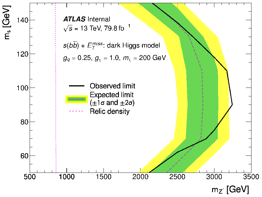
Now we’ll look at an example of how recast-atlas can be used: the monosbb recast. This ultimately produces exclusion contours over the model phase space, as seen here:

Full Simulation

There are many resources on the ATLAS tool chain, see e.g. this talk or the twiki. The most important aspect for recast-atlas is that all of the steps from generation up to derivation are handled by other atlas tools, so recast-atlas only handles the analysis stage, which essentially boils down to event selection and statistical analysis.

Therefore, if you wish to reinterpret an analysis, you’ll need to find out what derivation they used and create appropriate samples for your new signal model (note that you only need to worry about the signal; the backgrounds should already be included by the recast implementation of the analysis).

Depending on whether the analysis is in the recast catalogue or not, you may also need the analysis’ github repository for their recast implementation. In the example below, we’ll use the monohbb analysis, which is included in the recast catalogue.

Example

The next two subsections discuss the mono-Hbb analysis and dark Higgs model that together comprise the mono-Sbb re-interpretation.

Mono-Hbb Analysis

A Feynman diagram showing the leading-order contribution to production of dark matter in the mono-Hbb analysis. Z’ is a new mediator between the dark and visible sectors, which is coupled to a new pseudo-scalar Higgs boson A and a standard model Higgs boson h. A decays to two dark matter particles χ.

The Mono-H(bb) analysis searched for dark matter (DM) production in association with a Higgs boson decaying to two b-quarks from pp collision at a centre-of-mass energy of 13 TeV. The dataset was recorded by the ATLAS experiment in 2015 - 2017 and corresponds to an integrated luminosity of 79.8 fb^-1. The original results were interpreted using a Z’-2HDM signal model.

The signature of the search was:

1. MET (missing transverse energy) from the dark matter.
2. 2 b-tagged jets from the h decay.

The data was split into four bins based on MET. At high energies, the b jets become harder to resolve and ‘merge’ into a single ‘fat’ jet. Due to this, a different strategy was used in the ‘merged’ MET bin than was used in the three ‘resolved’ MET bins.

Additionally, several control regions were defined based on the number of isolated leptons. These control regions were then used in statistical analysis to constrain background parameters.

Dark Higgs Model

A leading-order Feynman diagram for the dark Higgs model in the mono-Sbb analysis. The similarity to mono-Hbb motivates re-interpretation.

For the mono-Sbb re-interpretation, a new dark Higgs signal model was used. In addition to Z’, the model introduces a Higgs mechanism in the dark sector that is responsible for the Majorana DM particle χ obtaining its mass. The dark Higgs mechanism results in a physical dark Higgs boson s. If s is lighter than χ, the DM relic abundance can be accounted for by χ→ss where s then decays to SM states. This also leads to processes (an example is shown above) that have similar experimental signatures to the mono-H analysis: MET from χ and two b-jets (with mass m_s instead of m_h).

The model has four free parameters: the mass of the particles m_χ, m_Z’, m_s and the coupling g_χ. In this re-interpretation, g_χ=1 (as was done in the Z’-2HDM model) and m_χ=200 GeV. Then, the signal grid is given by m_Z’∈[500, 3000] GeV in steps of 500 GeV and m_s∈[50, 110] GeV in steps of 20 GeV, resulting in a total of 24 points.

Running

There are two ways to run recast-atlas: locally (good for testing) or on lxplus (good for actual re-interpretations).

Local

To install recast-atlas locally, first setup a python virtual environment in whatever manner you prefer (conda, venv, etc.). Then, within that environment run:

pip install recast-atlas

lxplus

To use recast-atlas on lxplus, you need to ssh into a special lxplus node: ssh username@lxplus-cloud.cern.ch. Then, run:

source ~recast/public/setup.sh

In either case, if setup was successful then running recast --help should display usage information for recast-atlas.

The recast-monosbb workflow is available here. Running recast-atlas is quite straightforward and covered in the documentation. The README describes how to use several scripts to run the full signal grid; these scripts just run recast-atlas on every point in the signal grid. However, since it takes ~8 hours and significant computing resources, we won’t try it here.

Inputs

When doing a re-interpretation, it’s important to understand the structure of the analysis, so that you know what inputs you need to provide. In most cases, this should be documented as part of the preservation of the analysis. The mono-h(bb) workflow is fairly simple:

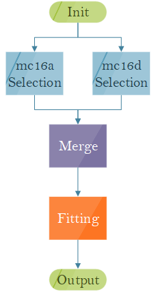
First, two selection stages for MC16A/D are run. Then, the results are merged and passed to a fitting stage. For these different stages, there are different inputs that we need to provide.

For the selection stages, we need (both for mc16a and mc16d):

• Monte Carlo simulation of the signal.
• Cross section.
• Luminosity.
• Pileup reweighting file.

For the fitting stage we need:

• Theory uncertainties for our signal.

recast-atlas expects a yaml file that specifies the inputs for a re-interpretation (more on this when we preserve our own analysis). For the mono-s(bb) re-interpretation, these are stored in the mono-sbb-config repository. Note that there is one file for each point in phase space.

Key Points

• recast-atlas utilizes full atlas simulation and can be used for the best reinterpretation accuracy.

• recast-atlas relies upon docker images and workflows that describe the existing analysis completely.